In the first article of this series I focused on a quick overview of iZotope Iris 2, I rapidly glanced at its interface and touched on some of the main functionality; it is now time to start working on an actual patch.
Before doing that we should first ask ourselves what is the goal we want to achieve with the new sounds. That is not to say that you should avoid experimenting and creating patches just by randomly move knobs and tweak sounds, this is where most of the inspiration is hiding after all! On the other end, giving us a concrete target, can set things straight for some decisions that are necessary to make early. For example, are we interested in creating a lush pad, an eerie alien sound from a distant planet, or perhaps an hunting deep and horrific drone? How much of the sound do we want to be pre-processed (end hence embedded in the actual sample file)? Do we want this pad to play nice at high intervals, more or less equally through the spectrum, or focused on the lower end?
The last question hides one interesting limitation with Iris, since it is not possible to map different samples to multiple keys in the same sample slot, unlike other samplers like Kontakt that allows you to have multiple velocity layers and multiple samples all over the keyboard. You can help this a bit by mapping the four samples at your disposal to different areas of the keyboard and restricting the play range, to avoid in part the side effect of extremely wide sample stretching – for example by having four main piano notes at four different octaves – but otherwise, whenever you play a sample that is rooted in C1 at C9, you are going to experience quite some glitchy noise. On the other end, this weakness also highlights that the best use case for Iris is not the ability to be used as a general sampler, but rather in its spectral shaping characteristic to find and highlight those glitches!
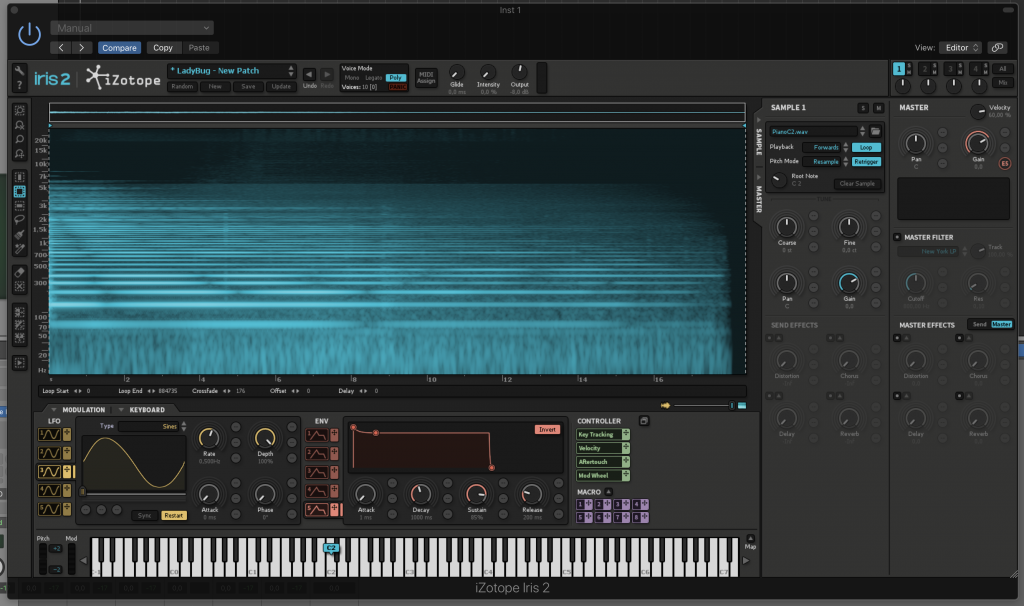
Let’s dive directly into it with a concrete example. For this article, we will be using a sample of a grand piano – I will attach that at the end of the article so you can experiment with it, together with the final patch. The very first thing is to start Iris of course, and then choose “New”, although Iris should already start with an empty patch. Drag and drop the “PianoC2.wav” sample into the first sample slot, the result should look like Fig. 1.
Iris should detect that the sample is rooted at C2, in case it doesn’t, select C2 in the “Root Note” knob in the sample section and play it (alternatively, you can drag the root note bubble on the keyboard to the right piano key). Save the patch by calling it “Iris2 – Patch Tutorial”, by taking mental note of the “category” in which the patch has been created. There is no immediate way to create a category, but it really is just a directory under the main library location, so you can create one by just adding a new directory there, for example: “/Library/Application Support/iZotope/Iris 2/Iris 2 Library/Patches/LadyBug”.
Did you save it? Fantastic, your first patch has been created and we’re done!
Well, yes, by default, this patch isn’t terribly exciting, so let’s add some spice to it. As I suggested before, it is now a good time to decide what kind of sound we’re after and for this tutorial, we will settle for a glitchy pad, since we love those.
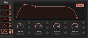
Before we start cutting the sample and adding interesting effects, let’s modify the master gain envelope, with a slower attack and a longer release, letting the sound die off more gradually over time; the master gain envelope is the E5, for now let’s choose 2 seconds for the attack time, 5 for the decay, 85% for the sustain, and then about 6 seconds release time, we may need to revisit this later and tweak the VCA, but for now this should give us plenty of space for our pad! We can also smooth out a bit the curve, by clicking and dragging the shape of the envelope outside of the control points of the ADSR, when done, yours should look more or less like mine in Fig. 2.
You can play some chords now, our patch is already a bit nicer, although we still have some work to do. To save it again, just press “Update”, this will overwrite the patch file with the new settings (be careful doing that with factory presets though!).
If you pay attention, the sample “loop” mode is on. This produces a nice plucked sound when the sample restarts, caused by the fact that the envelope affects the gain of the whole note as it is being played so when the sample loops it plays back at whatever gain is currently derived by E5. Additionally, since the note play at different speed (we kept the pitch mode on “resample”) the higher notes will loop faster than lower ones. This patch, as it is now, is very interesting, even if we didn’t do much Iris 2 specific, so let’s do some more processing.
You can always audition the modifications to the original file by clicking on the small icon at the very bottom of the tooling panel, on the left; this allows us to check how the customisation of the waveform at the root pitch sounds. As you can see from the spectrogram, there is quite a lot of harmonic overtones content present, this is a piano sample after all. C2 is the “great” or “low C”, two octaves below middle C – set at C4 on the keyboard, that is, the fourth C from the bottom – and with a centre frequency at about 65.4 Hz. You can see how much energy is present in this band, as well as in any of the other bands of the spectrum: the note was played with the sostenuto pedal pressed so there is lots of sympathetic resonance from the other strings and the soundboard with the note that doesn’t die off so easily being free to resonate naturally. The room also played its role of course, although we recorded in a sound proof place, it was quite small and there is still an audible bunch of reflections; it is difficult to “see” the reverb as it contributes to most of the same frequencies, but generally a reverb tail appears as shades that develops away from the main sound, like a blur on an instagram filter; here, this is not very significant and the overall sound is very nice, even with this one sample. I did clean up the sample a bit though, which can be seen from the lack of content in the upper end of the spectrum, this was mostly to remove the background noise of the portable recorder; it wasn’t prominent, but I wanted to prevent it from adding when playing multiple notes of the same sample, since the noise adds up pretty quickly. Since there wasn’t much tonal content in those frequencies anyway, I just cut most of it off, which is kind of the same effect that a low pass filter would achieve, although I used RX in this instance (incidentally, Iris shares parts of the same engine of RX for its spectral processing).
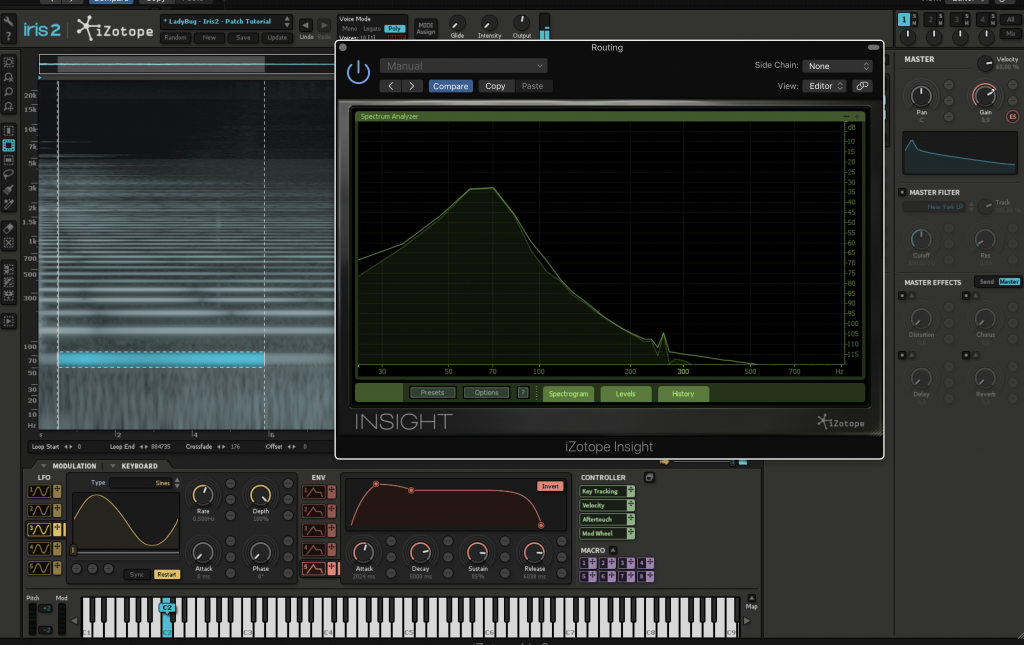
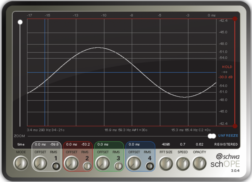
Now, one thing I like from Iris is that you have a very convenient spectrum analyser, although is not as accurate as a dedicated one, it is very useful to see what’s going on with the frequency over time as you play the notes, especially if you are using Iris as a standalone synth. Let’s now use the “Time and Frequency Selection Tool” to highlight a portion of the harmonic content, as in Fig.3, and see how it affects the sound. Unsurprisingly, as you can see – and hear – from the indeed more accurate Insight spectrogram, we are producing sound centred in the 65.4 Hz fundamental. In fact, if we check with an oscilloscope, we can see that this is indeed a sine wave with a period of a bit more than 15 milliseconds.
You can do the same for each and every overtone, just highlight in turn each of the horizontal areas that look brighter, those are the harmonic overtones, the first, second, third, and so on, try that now, the first overtone, which is the second harmonic – in the spectrogram the line just above our fundamental – is f*2, and it sits at 131 Hz, one octave above f; the second overtone, or f*3, is at 196.5 Hz, and is the fifth above this octave; the third overtone is two octave above the fundamental, f*4 or 327.5 Hz, and so on. Cool, we have confirmed that Fourier analysis works!
Another interesting thing to do, is to select one overtone and then play it at a different offset, for example select the fundamental (at C2) and then play it at C3, which is one octave above C2 of course: we are now producing a sine wave at about 131 Hz, the math works indeed!
What we’re doing here is to just let each overtone pass in isolation, but that alone is not very interesting, since we are removing all the character from the sound, all the non harmonic content that is between those overtones and that is specific of the instrument we are playing: we now have just a bunch of sine waves. But even so, with a bit of programming of the LFOs, we can use those “pure” sinusoids to create some very simple FM synthesis. Let’s try this out.
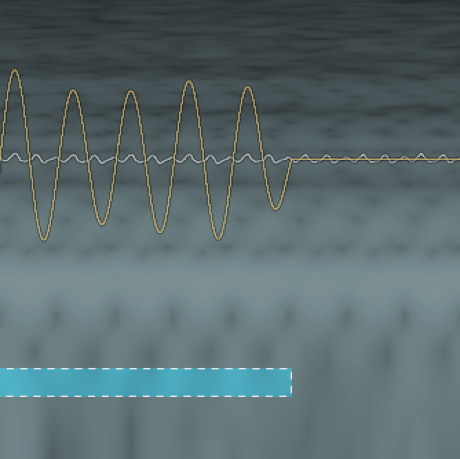
First of all, let’s fix the playback mode so that we have a continuous forward/backward loop. We should also get rid of some clicks and pops that now are being introduced by our slicing of the sample; there are two ways to achieve that, the first is to cut the sample at the zero cross point (where the waveform amplitude is exactly zero). You can make the waveform visible by moving the display blend slider toward the “waveform” setting, this is located just below the spectrogram, on the right side, and then zoom all the way in so that the individual wave cycles are visible, as in Fig. 5.
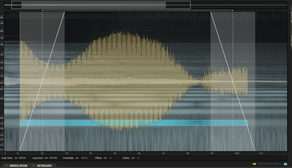
A better and more convenient alternative is to use the crossfade option to fade the loop, although this only helps for the very begin and the very end of the loop: if you have non continuous regions you need to tweak the start and end manually. Fig. 6 illustrates this second alternative.
Back to the FM Synthesis, but what it is exactly? “Simply” put, and it’s in quote because this type of synthesis is anything but simple, Modulation Synthesis is the ability to modulate a waveform that carries information, called, well, carrier, with another waveform, called, you guessed it, modulator. This form of synthesis is called FM when the modulator changes the frequency of the carrier signal (Frequency Modulation), it is called AM synthesis when it changes the amplitude (Amplitude Modulation), or Ring Modulation, which is a kind of Amplitude Modulation, where the carrier signal is multiplied with the modulator signal resulting in an alternating phasing effect and the typical metallic sound. Iris is not a perfect FM synthesiser, you would need a modulator that can produce higher frequency oscillations to be properly useful, while the LFOs we have at our disposal arrives at most at 50 Hz, which is enough for achieving some interesting effects (including all sorts of tremolo, chorus and phasing) but not so much for actual sound synthesis. We do have, however, a few waveforms that can be used specifically for FM synthesis, under the Multiply sections of the LFOs. It’s still not a DX7, but does it matter? Actually, the most important functionality here is the ability to alter the audible spectrum of a signal, let’s then combine the LFOs to modulate the pitch with some more spectral synthesis to see what we get.
Let’s highlight some more frequencies, let’s say roughly a rectangle between 700 to 130, with the same length of the lower harmonic. Add the LFO 1 modulation source to the Fine Tuning of the first sample and select “Sine M” from the Multiply menu. Let’s use a couple more modulation sources, Env1, LFO2 and Env2 to modulate the shape of the LFO, combining the first two modulation to “Mult” and the second two as “Add”. For Env1 and Env2 we can use a shape with a slow attack and a slow decay, while for LFO2 let’s just use a simple sine wave. Finally, let’s modulate LFO1 rate with Env1. Uh, lots of changes, but no worries if you are lost, I’m going to share the patch in a minute so you can import it in your session and study all the details. You should now have something that sounds like a very glitchy organ, especially at higher frequencies.
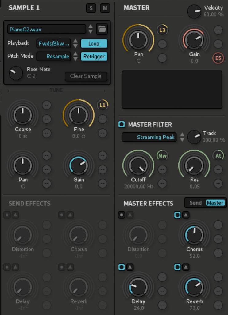
Let finish the patch with some effects, delay reverb and chorus. You may experiment with more of the modulation sources, for example to pan the sound. A final touch is add some modulation wheel, aftertouch and velocity control to the filters, this way the patch changes based on the dynamics of your playing, like shown in Fig. 7. You can also try to experiment with the LFO by adding key tracking to dynamically alter the carrier pitch as you play.
Ok, as promised, here is the patch, just follow the link, the license as usual is a very permissive Creative Commons Attribution 4.0 International License.